Chapter 2
Platform Overview

2.1 MRiLab Simulation Platform

The MRiLab simulation platform consists of

1. A Main Simulation Control Console
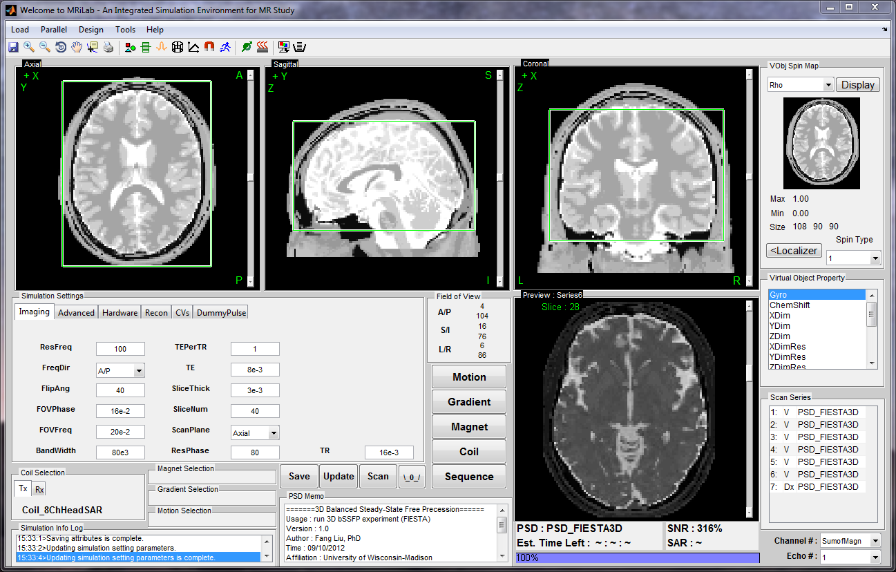
   The main simulation console (Figure 2.1) behaves analogous to a MR scanner console for graphically adjusting imaging setup and conducting simulation control. Simulation feedback are instantly updated on information panels during simulation.

   ---

   
   

   Figure 2.1: The MRiLab Main Simulation Control Console. This control console functions like a MR scanner console for graphically adjusting imaging setup and conducting simulation control.

   ---

2. Design Toolboxes
   The Design toolboxes (Figure 2.2) provide independent interfaces for analyzing RF pulse (e.g. SLR, non-adiabatic and adiabatic pulse etc.), constructing arbitrary pulse sequence (e.g. SPGR, SSFP and FSE etc.), configuring coil profile and static field (i.e. B1+/- and B0 field), designing imaging object moving track and evaluating spatial specific absorption rate (SAR). Dedicated image display and analysis tools (SpinWatcher, SARWatcher, MatrixUser and arrayShow) are developed and tailored to work with multi-dimensional image array output.

   ---

   
   

   Figure 2.2: The Shortcut for Function Toolbox on Simulation Control Console. Each icon is associated with an individual toolbox with specific functions.

   ---

3. Discrete Bloch-equation Solving Kernels
   The Bloch-equation solving kernels manipulate tissue spin evolution at discrete time interval with a desired spin model and at a given MR sequence. These kernels are accelerated using Matlab MEX functions that are optimized for running GPU and multi-threading CPU parallel computing techniques. Moreover, these kernels are also capable of preprocessing acquired MR signal and k-space locations prior to desirable image reconstruction. Further image reconstruction with stored k-space data is accomplished in corresponding reconstruction module.
4. Macro Library
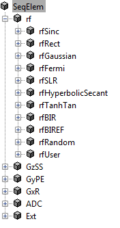
   MRiLab uses a concept of macros for simplifying experiment design. A macro in MRiLab is defined as a programming-free module that can be added, removed and modified in the process of constructing MR sequence, coil profile, magnet field and object moving track, etc. For instance, a Sinc RF pulse (rfSinc) is considered as a RF macro that can be used for constructing a gradient echo sequence, and the attributes of this macro include pulse starting time (tStart), pulse ending time (tEnd) and the time bandwidth product (TBP) etc. MRiLab provides a macro library (Figure 2.3) covering a wide range of macros. Using these predefined macros, you should be able to accomplish most of experimental design work. However, if special macros are needed, MRiLab also provides interfaces to work with user-defined macros. More detailed description for macros is provided in Chapter 5.

   ---

   
   

   Figure 2.3: The Macro Library Tree Structure in MRiLab. Individual tree nodes under SeqElem root are functional macros that can be used for designing MR sequences. Notice that only RF nodes are unfolded here for display purpose.

   ---

MRiLab applies flexible simulation information storage by using XML file system, which simplifies translating simulation across different studies. MRiLab also supports external plugins programmed using either Matlab or C language for creating extendable simulation environment.

2.2 Simulation Workflow

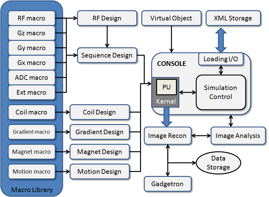
The workflow diagram of MRiLab simulation is shown in Figure 2.4. One typical simulation requires input of :

• Virtual object (VObj) with specific tissue properties including Rho (spin density), T1 and T2 etc.
• MR sequence to drive spin evolution
• B1+/- field for RF transmitting and receiving, default to be uniform field
• Gradient field for spatial encoding, default to be linear gradient
• Magnet field perturbation describing main static field inhomogeneity (dB0), default to be zero
• Motion pattern for describing imaging object movement during real time simulation

The input is configured at the main control console where the user can modify any aspect of the simulation experiment. The main console preprocesses the input information, then translates them into kernel signal, based on which the discrete solving kernel executes each voxel of imaging objects with either GPU or multi-threading CPU acceleration. The acquired MR signal k-space data from the kernel passes to image reconstruction module where either default recon code or external recon tool (e.g. Gadgetron) is applied. The reconstructed image can be analyzed using MRiLab image display tools including :

• MatrixUser : An image display and analysis tool for manipulating multidimensional matrix
• SpinWatcher : An analysis tool for analyzing spin evolution behavior within a single voxel
• SARWatcher : An analysis tool for analyzing local spatial SAR distribution
• arrayShow : A Matlab image viewer for the evaluation of multidimensional complex images

2.3 Gradient Echo: Start A Simple Scan

Up to this point, you may wonder how I can start to use MRiLab. Here below is a simple 3D Gradient Echo (GRE) simulation example to gain your first experience of using MRiLab.

• Open MRiLab by running ‘MRiLab.m’ under the root folder. MRiLab will try to detect available CPU and GPU devices, and initialize the simulation environment. After initialization (typically in couple seconds), MRiLab Main Simulation Control Console will open. Empty Axial, Sagittal, Coronal and Preview views show up. Notice that on the console, several push buttons are disabled at this point, it means more inputs are needed for activating them.
• To simulate images, the virtual object a.k.a. digital phantom is needed. Go to ‘Load’, ‘Load Phantom Example’, choose one of the predefined digital phantoms for the experiment. Several digital phantoms suitable for different experiment purposes are already provided. Here, let’s choose ‘Brain (Standard Resolution 108x90x90)’. After loading this phantom, notice that preview images show up at the top right corner under ‘VObj Spin Map’. The property information of this phantom also show in ‘Virtual Object Property. Let’s choose ‘Rho’ map from the pop-up menu, and click ‘Localizer’ button to show more image details. Now Axial, Sagittal and Coronal axes are displayed with this 3D digital phantom. Click ‘Update’ button to accept this phantom loading. Notice that after updating, all push buttons become enabled.
• Since we want to simulate 3D GRE experiment, we need to load 3D GRE sequence first. Click the ‘Sequence’ button located at the center portion of the console. A SeqList will open where you can choose and load MR sequences. Let’s click ‘Dimension’ pop-up menu and choose ‘3D’. The Category list shows a full list of current available sequence type. Click ‘GradientEcho’, then click ‘PSD_GRE3D’ from the Sequence list. Click ‘Accept’ button to accept and load a 3D GRE sequence. Notice that the ‘Simulation Settings’ tabs on the console update and change to the setting for the current GRE sequence. Click ‘Update’ button to accept this sequence loading.
• Under the ‘Imaging’ tab, there are several parameters for imaging control, for instance, Field-of-View in the frequency encoding direction (FOVFreq). We can simply accept the default setting at this moment, however, if you do make any changes, you need to click ‘Update’ button to update those changes before proceeding to Scan.
• The final step is to click ‘Scan’ button and wait for the simulation to start. Depending on imaging setting and computing hardware, the simulation will typically finish in a short period of time, the reconstructed image will show in the ‘Preview’ view.

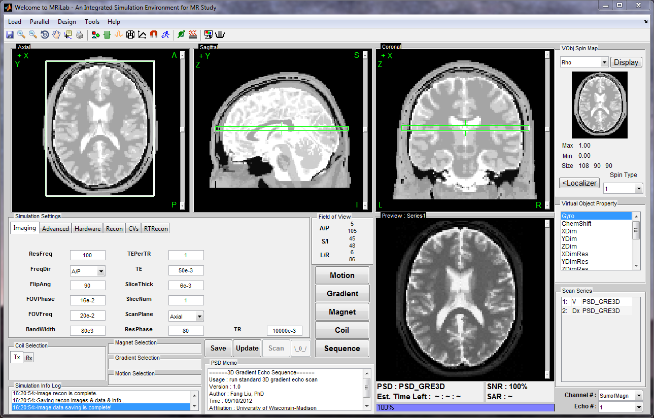
The final result of this 3D GRE experiment should be somewhat similar to this (Figure 2.5).

If you managed to simulate this gradient echo image, congratulations! You have successfully performed your first MRiLab experiment. So you should be prepared for deeper understanding of MRiLab simulation platform by following the rest of this user guide.