Chapter 7
MRiLab Applications
This chapter shows a few examples for demonstrating the applications of MRiLab
simulation
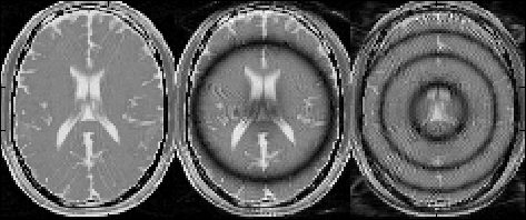
7.1 bSSFP with Non-uniform B0
This example (Figure 7.1) simulates the dark banding artifact in bSSFP images
arisen from non-uniform B0 field. To perform this simulation, the following steps are
needed:
- Load Brain (Standard Resolution 108 × 90 × 90)
- Load PSD_FIESTA3D
- Load Mag_GaussianHead
The user can adjust the ‘FlipAng’, ‘TR’ and ‘TE’ to modify the pattern of the
banding artifact.
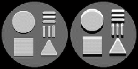
7.2 Fat Chemical Shift
This example (Figure 7.2) simulates chemical shift artifact at the interface of water
and fat in a GRE sequence. To perform this simulation, the following steps are
needed:
- Load Water Fat Phantom (256 × 256 × 32 × 2)
- Load PSD_GRE3D
The user can adjust the ‘BandWidth’ and ‘FreqDir’ to modify the appearance of
the chemical shift.
7.3 Multi RF Transmitting
This example (Figure 7.3) simulates multiple RF transmitting using a bSSFP
sequence. To perform this simulation, the following steps are needed:
- Load Brain (Standard Resolution 108 × 90 × 90)
- Load PSD_FIESTA3D
- Load Coil_8ChHead to Tx
- Set ‘MultiTransmit’ to ‘on’
The user can adjust the ‘B1Level’ to modify the actual flip angle, modify the RF
pulse using MR sequence Design Toolbox for individual RF source, or modify the coil
configuration for generating desired B1+ field.
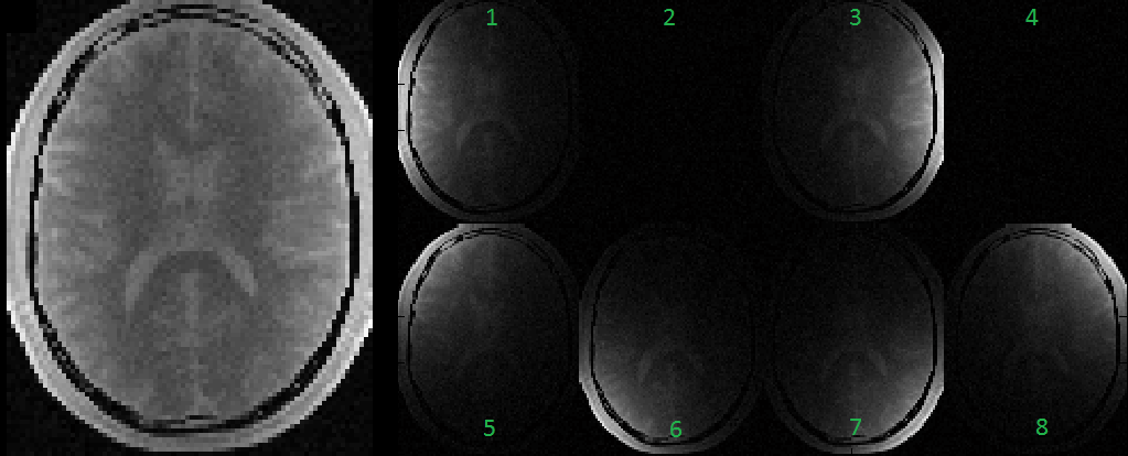
7.4 Multi Receiving Coil
This example (Figure 7.4) simulates multiple receiving using a SE sequence. To
perform this simulation, the following steps are needed:
- Load Brain (Standard Resolution 108 × 90 × 90)
- Load PSD_SE3D
- Load Coil_8ChHead to Rx
The user can adjust the coil configuration for generating desired B1-
field. All eight channels will be receiving MR signal from the virtual object
individually.
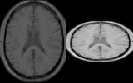
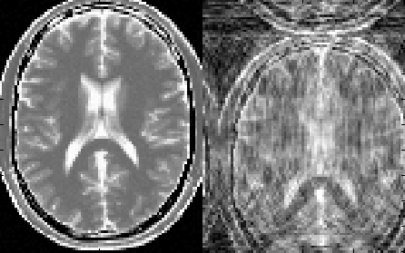
7.5 Image Gradient
This example (Figure 7.5) simulates applying non-unit gradient with a 3D SPGR
sequence. To perform this simulation, the following steps are needed:
- Load Brain (Standard Resolution 108 × 90 × 90)
- Load PSD_SPGR3D
- Load Grad_LinearHead
The user can adjust the gradient structure for generating desired gradient field.
Notice that this applied gradient in GyPE GradLine has a factor of 0.5 in the Y
direction. This will cause image contraction in the Y direction.
7.6 Motion Artifact
This example (Figure 7.6) simulates motion artifact with a 3D GRE sequence. To
perform this simulation, the following steps are needed:
- Load Brain (Standard Resolution 108 × 90 × 90)
- Load PSD_GRE3D
- Load Mot_ShiftHead
The user can adjust the motion structure to generate different motion track
patterns, and/or modify motion triggering in the Ext sequence line to sample object
movement.